Chapter three: The weighted boilerplate cost of majuscule (WACC)
Affiliate learning Objectives
Upon completion of this chapter you lot will be able to:
- calculate a cost of disinterestedness using Dividend Valuation Model (DVM), the Capital Asset Pricing Model (CAPM) and Modigliani and Miller's Suggestion 2 formula.
- calculate a price of debt using DVM, CAPM and credit spreads.
- sympathise how lenders set their interest rates on debt finance.
- calculate a weighted average cost of capital.
- understand the circumstances in which the WACC can be used every bit a project discount rate.
1 The weighted boilerplate cost of capital (WACC)
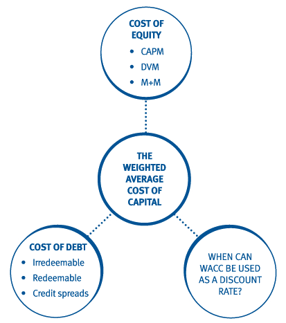
Overview of the WACC
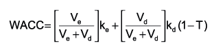
A key consideration in fiscal management is the firm's WACC. TheWACC is derived by finding a business firm's cost of equity and cost of debt andaveraging them according to the market place value of each source of finance.The formula for calculating WACC is given on the examination formula canvass equally:

 Caption of terms
5east and 5d are the market values of equity and debt respectively.
ke and kd are the returns required by the equity holders and the debt holders respectively.
T is the corporation tax charge per unit.
thousanddue east is the cost of equity.
kd(1-T) is the cost of debt.

This chapter reviews the basic techniques for deriving price ofequity and cost of debt from the F9 paper, and adds some more advancedtechniques too.
2 The cost of equity (ke)
Methods of calculating grande
The three main methods of calculating keast are:
- the Capital Asset Pricing Model (CAPM)
- the Dividend Valuation Model (DVM)
- Modigliani and Miller'southward Proffer ii formula
The formulae for these methods are all given on the exam formula canvass.
The Majuscule Asset Pricing Model (CAPM)
The CAPM derives a required render for an investor by relatingreturn to the level of systematic take a chance faced past an investor - note thatthe CAPM is based on the assumption that all investors are welldiversified, so only systematic gamble is relevant.
The CAPM formula is:
Required return ( ke ) = Rf + ßi (E(Rgrand) - Rf)
where:
Rf = take chances free rate
Eastward(Rg) = expected return on the market
N.B. (Eastward(Rthousand) - Rf) is called the disinterestedness risk premium
ßi = beta factor = systematic risk of the house or project compared to market place.
The portfolio effect
The CAPM model is based upon the assumption that investors are welldiversified, so will have eliminated all the unsystematic (specific)adventure from their portfolios. The beta factor is a measure of the level ofsystematic risk (general, market run a risk) faced by a well diversifiedinvestor - see more than details on beta factors below.
The risk reduction through diversifying is known as the portfolio effect.
If an investor is not well diversified, the level of risk affectingthe investor can be calculated using the 2 asset portfolio formula:
Overall take a chance (standard divergence) = (wa twosa 2+wb 2s b ii+2wawbrabdue southasouth b)½
where
westwarda and wb are the proportions invested in two investments a and b
southwarda and sb are the risks associated with investments a and b (standard deviations)
rab is the correlation coefficient of the investments a and b
The beta gene
The beta gene indicates the level of systematic risk faced past an investor.
A beta > 1 indicates in a higher place average risk, while beta < 1="" means="" relatively="" depression="">
Beta factors are derived by statistically analysing returns from aparticular share over a period compared to the overall market returns.If the returns on the private share are more than volatile than theoverall market, the firm's beta will be greater than 1.
Illustration of the use of the CAPM formula
Gillespie Co has a beta gene of 1.73. The electric current render on arisk complimentary nugget is three% per annum and the equity run a risk premium is 12%.
Hence, using CAPM, Gillespie Co'south price of equity (render required by the shareholders) is
3% + (1.73 × 12%) = 23.76%.
Which beta factor to apply?
To summate the current toll of equity of a house, the current beta gene tin exist used.
However, if the firm's electric current beta cistron cannot be derived easily, a proxy beta may exist used.
A proxy beta is normally establish past identifying a quoted company with asimilar business take a chance profile and using its beta. Yet, whenselecting an appropriate beta from a like company, account has to betaken of the gearing ratios involved.
The beta values for companies reverberate both:
- business risk (resulting from operations)
- finance take a chance (resulting from their level of gearing).
There are therefore 2 types of beta:
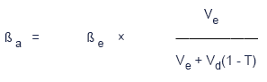
- “Asset†or “ungeared†beta, ßa , which reflects purely the systematic adventure of the business organisation expanse.
- “Equity†or “geared†beta, ßeast , which reflects the systematic risk of the concern area and the company specific gearing ratio.
In the examination, you will oftentimes have to degear the proxy equity beta(using the gearing of the quoted company) and and so regear to reflect thegearing position of the company in question.
The formula to regear and degear betas is:
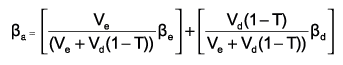
However, ßd (beta value for debt) is ofttimes assumed tobe zero, considering of the low hazard of being a debt holder, so thisequation oft simplifies to give
 Examination your agreement i
The directors of Moorland Co, a company which has 75% of itsoperations in the retail sector and 25% in manufacturing, are trying toderive the firm's cost of equity. However, since the company is notlisted, information technology has been difficult to determine an advisable beta gene.Instead, the following information has been researched:
Retail industry - quoted retailers have an average equity beta of ane.20, and an average gearing ratio of 20:80 (debt:equity).
Manufacturing industry - quoted manufacturers have an boilerplate equity beta of 1.45 and an average gearing ratio of 45:55 (debt:disinterestedness).
The risk complimentary rate is 3% and the equity chance premium is 6%. Taxation oncorporate profits is 30%. Moorland Co has gearing of 50% debt and 50%equity by market values. Assume that the risk on corporate debt isnegligible.
Required:
Calculate the cost of equity of Moorland Co using the CAPM model.
The dividend valuation model (DVM)
Theory: The value of the visitor/share is the present valueof the expected future dividends discounted at the shareholders’required charge per unit of return.
Assuming a constant growth charge per unit in dividends, g:
P0 = D0(1 + g) / (ke - yard)
(this formula is given on the formula sheet)
Explanation of terms
D 0 = electric current level of dividend
P 0 = current share price
thou = estimated growth charge per unit
If nosotros need to derive ke the formula can be rearranged to:
ke = [D0 (1+k) / P0 ] + g
Illustration of the DVM formula
Cocker Co has just paid a dividend of 14 cents per share. In recentyears, annual dividend growth has been 3% per annum, and the currentshare price is $1.48.
Using the DVM formula, the cost of equity is [0.14 × i.03 / one.48] + 0.03 = 12.vii%
Deriving g in the DVM formula
There are two means of estimating the likely growth rate of dividends:
- Extrapolating based on past dividend patterns.
- Bold growth is dependent on the level of earnings retained in the business.
Estimating dividend growth from past dividend patterns
This method assumes that the past blueprint of dividends is a fair indicator of the future.
The formula for extrapolating growth can therefore be written as:

where:
due north = number of years of dividend growth
This method can simply be used if:
- recent dividend pattern is considered typical
- historical pattern is expected to proceed.
As a result, this method will unremarkably only exist appropriate to predict growth rates over the brusk term.
Analogy of the calculation
A company currently pays a dividend of 32¢; five years ago the dividend was 20¢.
Estimate the annual growth rate in dividends.
Solution
Since growth is assumed to be constant, the growth rate, g, can beassumed to accept been the aforementioned in each of the 5 years, i.e. the 20¢ willhave get 32¢ after 5 years of constant growth.
20¢ × (1 + g)5 = 32¢
or (1 + chiliad)5 = 32/20 = i.6
1 + yard = 1.61/five ≈ ane.one, so k = 0.1 or 10%.
Estimating growth using the earnings memory model (Gordon’s growth model)
This model is based on the assumption that:
- growth is primarily due to the reinvestment of retained earnings
The formula is therefore:
m = r × b
where:
b = earnings retention rate
r = rate of return to disinterestedness
What is r?
At F9 level, r was considered to be the Accounting Rate of Return on equity calculated equally:
r = PAT / opening shareholders' funds
Nonetheless, at P4 we need to re-examine this supposition. The weakness of the ARR as a measure out of return is that:
- it ignores the level of investment in intangible avails
- in the long run, the return on new investment tends to the cost of disinterestedness.
Hence, if a short term growth rate is required, the ARR provides afair approximation for use in the growth model. Even so, if a long termgrowth rate is needed, grande should exist used as the percentage return. To avoid a recursion problem, this should be derived using CAPM.
Modigliani and Miller's Proposition 2 formula
Modigliani and Miller's gearing theory is covered in the later on chapter on Upper-case letter Structure and Financing.
Equally role of their theory, they derived a formula which can be used to derive a firm's cost of equity:
ke = keast i + (1-T)(ke i - kd )(Vd / Ve)
(this formula is given on the formula sail)
Explanation of terms
Ve and Vd are the market values of disinterestedness and debt respectively.
kd is the (pre taxation) render required past the debt holders.
T is the corporation tax charge per unit.
thoueast i is the cost of equity in an equivalent ungeared firm.
keast is the cost of equity in the geared business firm.
Test your understanding 2
Moondog Co is a company with a 20:80 debt:disinterestedness ratio. Using CAPM, its cost of equity has been calculated as 12%.
Information technology is considering raising some debt finance to alter its gearingratio to 25:75 debt to disinterestedness. The expected return to debt holders is 4%per annum, and the rate of corporate tax is thirty%.
Summate the theoretical cost of disinterestedness in Moondog Co after the refinancing.
3 The price of debt
Methods of calculating toll of debt
The company's cost of debt is found by taking the return required past debt holders / lenders (yardd) and adjusting it for the tax relief received by the firm equally it pays debt interest.
Note on exam terminology
In test questions you may exist given the toll of debt or you may accept to calculate it - see below for calculations.
If you are given the "price of debt", be enlightened that the cost of debtis unremarkably quoted pre-tax because this is the charge per unit at which thecompanies volition pay interest on their borrowings (even though the 'truthful'cost to them will be cyberspace of tax considering interest is payable before taxand therefore companies do good from the 'revenue enhancement shield').
It can be assumed, therefore, that cost of debt will mean pre-tax cost of debt (thousandd) unless it is clearly stated otherwise.
Using the DVM to estimate cost of debt
In paper F9, the cost of debt was more often than not estimated using the principles of the dividend valuation model.
The use of DVM to judge cost of debt
As seen to a higher place, the basic theory of the DVM is:
The value of a share = the nowadays value of the hereafter dividends discounted at the shareholders' required rate of return
Using the same logic,
The value of a bond = the present value of the future receipts(interest and redemption amount) discounted at the lenders' requiredrate of return.
This theory gives rise to two alternative calculations of kd (1-T):
Post tax cost of debt
Irredeemable debt
Yardd (1-T) = I (one-T) / MV
where
I = the almanac involvement paid,
T = corporation tax rate,
MV = the current bond price.
Illustration of method
Mackay Co has some irredeemable, 5% coupon bonds in issue, which are trading at $94.l per $100 nominal. The tax charge per unit is 30%.
Mackay Co'due south postal service tax price of debt is 5(i-0.xxx) / 94.l = 3.7%
Redeemable debt
thousandd (one-T) = the Internal Charge per unit of Render (IRR) of
- the bond price
- the involvement (net of revenue enhancement)
- the redemption payment
Analogy of method
Dodgy Co'southward 6% coupon bonds are currently priced at $89%. The bondsare redeemable at par in 5 years. Corporation tax is thirty%. Summate thepost tax price of debt.
To calculate IRR, nosotros discount at 2 rates (v% and ten% hither) and so interpolate:
PV at five% = 89 - (6(one-0.30) × five yr 5% annuity factor) - (100 × 5 year 5% discount factor) = -7.58
PV at 10% = 89 - (6(i-0.30) × 5 yr ten% annuity factor) - (100 × five twelvemonth ten% discount gene) = 10.98
Hence IRR (post revenue enhancement toll of debt) is approximately vi%
Pre tax toll of debt (or "yield" to the debt holder)
In both the previous examples, the focus was on finding the posttax price of debt, which is a key component in the company's WACCcalculation.
In social club to compute the pre taxation cost of debt (sometimes called the yield to the investor) the method is very similar.
For irredeemable debt, the pre tax cost of debt is simply I/MV.
For redeemable debt, the pre tax price of debt is the IRR of thebond price, the GROSS interest (i.e. pre tax) and the redemptionpayment.
In both cases, the only deviation from the to a higher place calculations is that interest is now taken pre revenue enhancement in the formulae.
Credit spread
All the same, the main technique used in Paper P4 for deriving price of debt is based on an awareness of credit spread (sometimes referred to as the "default run a risk premium"), and the formula:
kd (1-T) = (Gamble complimentary charge per unit + Credit spread) (1-T)
The credit spread is a measure of the credit risk associated with acompany. Credit spreads are generally calculated by a credit ratingagency and presented in a tabular array like the i below: To understand howcredit spreads are derived, see the section on how lenders set theirinterest rates at the finish of this chapter.
Credit chance, rating agencies and spread
What is credit gamble?
Credit or default risk is the doubt surrounding a firm’s power to service its debts and obligations.
It can exist divers as the risk borne by a lender that the borrowerwill default either on interest payments, the repayment of the borrowingat the due engagement or both.
The function of credit rating agencies
If a company wants to assess whether a house that owes them coin islikely to default on the debt, a key source of information is a creditrating agency.
They provide vital information on creditworthiness to:
- potential investors
- regulators of investing bodies
- the business firm itself.
The assessment of creditworthiness
A large number of agencies can provide information on smallerfirms, but for larger firms credit assessments are usually carried outby one of the international credit rating agencies. The 3 largestinternational agencies are Standard and Poor's, Moodys and Fitch.
Certain factors have been shown to have a item correlationwith the likelihood that a company will default on its obligations:
- The magnitude and strength of the company’south cash flows.
- The size of the debt relative to the asset value of the business firm.
- The volatility of the firm’s asset value.
- The length of time the debt has to run.
Using this and other information, firms are scored and rated on a scale, such equally the one shown hither:
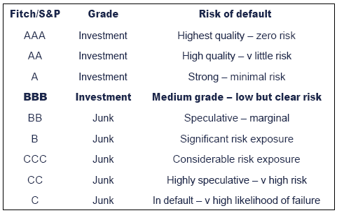
Calculating credit scores
The credit rating agencies use a diversity of models to assess the creditworthiness of companies.
In the popular Kaplan Urwitz model, measures such as firm size,profitability, blazon of debt, gearing ratios, interest cover and levelsof gamble are fed into formulae to generate a credit score.
These scores are and so used to create the rankings shown above. For case a score of above vi.76 suggests an AAA rating.
Credit spread
At that place is no way to tell in advance which firms volition default ontheir obligations and which won’t. As a result, to compensate lendersfor this uncertainty, firms generally pay a spread or premium over therisk-gratuitous rate of interest, which is proportional to their defaultprobability.
The yield on a corporate bond is therefore given by:
Yield on corporate bail = Yield on equivalent treasury bond + credit spread
Table of credit spreads for industrial visitor bonds:

Examples of calculations of yield
Uncomplicated analogy
The current return on 5-yr treasury bonds is three.half dozen%. C plc hasequivalent bonds in event but has an A rating. What is the expectedyield on C’s bonds?
Solution
From the table the credit spread for an A rated, five-year bail is 65.
This ways that 0.65% must be added to the yield on equivalent treasury bonds.
And then yield on C’due south bonds = 3.6% + 0.65% = 4.25%.
More advanced analogy
The current return on 8-year treasury bonds is four.2%. Ten plc hasequivalent bonds in issue just has a BBB rating. What is the expectedyield on X’due south bonds?
Solution
From the table the credit spread for a BBB rated, vii-year bond is 126. The spread for a 10-year bond is 149.
This would propose an adjustment of
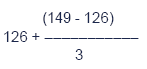
= 126 + 7.67 = 133.67
So one.34% must exist added to the yield on equivalent treasury bonds.
And then yield on X’s bonds = 4.ii% + 1.34% = 5.54%
Test your understanding 3
The current return on 4-year treasury bonds is 2.6%. F plc has equivalent bonds in issue merely has a AA rating.
(i) calculate the expected yield on F’s bonds
(ii) find F’s post tax cost of debt associated with these bonds if the charge per unit of corporation tax is xxx%
(Use the information in the table of credit spreads above).
Exam your understanding 4
Landline Co has an A credit rating.
It has $30m of 2 year bonds in issue, which are trading at $90%, and $50m of x year bonds which are trading at $108%.
The risk free rate is 2.5% and the corporation taxation charge per unit is thirty%.
Calculate the company's mail revenue enhancement cost of debt capital.
(Use the data in the tabular array of credit spreads to a higher place).
Using the CAPM to calculate cost of debt
The CAPM can be used to derive a required return every bit long as thesystematic hazard of an investment is known. Before in the chapter we sawhow to use an equity beta to derive a required return on equity. Wealso said that the risk on debt is usually relatively depression, and then the debtbeta is often zero. However, if the debt beta is not null (for exampleif the company's credit rating shows that information technology has a credit spread greaterthan zip) the CAPM tin can also exist used to derive grandd as follows:
kd = Rf + ßdebt (E(Rone thousand) - Rf)
Then, the post revenue enhancement toll of debt is kd (1-T) equally usual.
Test your agreement 5: WACC
An entity has the following data in its rest sheet (statement of financial position):
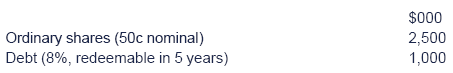
The entity's equity beta is i.25 and its credit rating according toStandard and Poor's is A. The share price is $1.22 and the debentureprice is $110 per $100 nominal.
Extract from Standard and Poor's credit spread tables:

The risk costless rate of involvement is 6% and the disinterestedness risk premium is 8%. Taxation is payable at 30%.
Required:
Summate the entity's WACC.
Awarding of Macauley duration to debt
In Chapter 2, we saw how to summate the Macauley Elapsing of aninvestment project. The method can also be used to measure thesensitivity of a bond's price to a change in interest rates.
Elapsing is expressed equally a number of years. The bigger the duration, the greater the gamble associated with the bail.
Illustration of Macauley Duration calculation for a bail
Tyminski Co has some x% coupon bonds in issue. They are redeemableat par in 5 years, and are trading at $97.25%. The yield (pre tax costof debt) is 10.743%.
The Macaulay Duration is calculated equally follows:
Step ane: Calculate the present value of each futurity receipt from the bail, using the pre taxation cost of debt as the discount rate.

Step two: Calculate the sum of (time to maturity x PV of receipt)
(ane × ix.03) +(2 × 8.15) +(three × vii.36) +(4 × half-dozen.66) +(5 × 66.05) = 404.30
Stride 3: Divide this by the total PV of receipts (i.east. the bond toll) to give the Macauley Duration.
Macauley Duration = 404.30 / 97.25 = iv.157 years
The longer the Macauley Duration, the more volatile the bond.
Benefits and limitations of elapsing
Benefits
- Elapsing allows bonds of dissimilar maturities and coupon rates to be compared. This makes decision making regarding bond finance easier and more effective.
- If a portfolio of bonds is synthetic based on weighted average duration, it is possible to identify the alter in value of the portfolio as involvement rates alter.
- Managers may be able to reduce interest rate risk past changing the overall duration of the bond portfolio (eastward.grand. past calculation shorter maturity bonds to reduce elapsing).
Limitations
The main limitation of duration is that it assumes a linearrelationship between involvement rates and bond cost. In reality, therelationship is probable to be curvilinear. The extent of the deviationfrom a linear human relationship is known as convexity. The more convexthe relationship betwixt interest rates and bond toll, the moreinaccurate elapsing is for measuring involvement rate sensitivity.
Further information on convexity
The sensitivity of bond prices to changes in interest rates isdependent on their redemption dates. Bonds which are due to be redeemedat a later engagement are more price-sensitive to involvement rate changes, andtherefore are riskier.
Duration measures the boilerplate time it takes for a bond to pay itscoupons and primary and therefore measures the redemption flow of abond. Information technology recognises that bonds which pay college coupons effectivelymature ‘sooner’ compared to bonds which pay lower coupons, even ifthe redemption dates of the bonds are the aforementioned. This is considering a higherproportion of the college coupon bonds’ income is received sooner.Therefore these bonds are less sensitive to involvement rate changes andwill take a lower duration.
Duration can exist used to assess the alter in the value of a bond when interest rates change using the post-obit formula:
Î"P = [â€"D x Î"i × P]/[1 + i],
where P is the cost of the bond, D is the duration and i is the redemption yield.
Yet, duration is just useful in assessing small changes in interest rates because of convexity.Every bit interest rates increase, the price of a bail decreases and viceversa, but this decrease is non proportional for coupon paying bonds,the relationship is not-linear. In fact, the human relationship between thechanges in bail value to changes in interest rates is in the shape of aconvex curve to origin, see below.

Duration, on the other hand, assumes that the relationship between changes in interest rates and the resultant bond is linear.
Therefore duration will predict a lower cost than the actual priceand for big changes in interest rates this difference tin can besignificant. Duration can only be practical to mensurate the approximatechange in a bond toll due to involvement changes, merely if changes ininterest rates practise not lead to a alter in the shape of the yield bend.This is because it is an average measure based on the gross redemptionyield (yield to maturity). However, if the shape of the yield curvechanges, elapsing can no longer be used to appraise the change in bondvalue due to involvement rate changes.
four How practice lenders ready their interest rates?
Link to credit spreads
The tabular array of credit spreads shown in a higher place showed the premium overrisk free rate which a visitor would have to pay in order to satisfy itslenders. Another way of looking at the issue of yield on a bond is tolook at it from the perspective of the lender. How lenders gear up theirinterest rates was the subject field of an article written past Bob Ryan forStudent Accountant mag in August 2008.
Overview of the method
Lenders ready their interest rates later assessing the likelihoodthat the borrower will default. The basic thought is that the lender willassess the likelihood (using normal distribution theory) of the firm'scash flows falling to a level which is lower than the required interestpayment in the coming twelvemonth. If it looks likely that the business firm will haveto default, the interest rate will exist set at a loftier level to compensatethe lender for this risk.
Introduction to normal distribution theory
The exam formula sail contains a normal distribution tabular array. Normal distributions accept several applications in the P4 syllabus.
A normal distribution is ofttimes fatigued as a "bell shaped" curve, with its top at the mean in the centre, as shown:
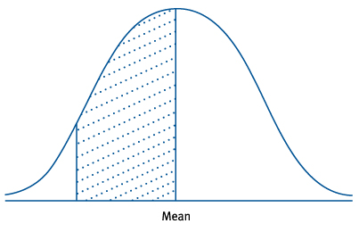
The effigy from the normal distribution table gives the size of anarea (shaded on the diagram) betwixt the mean and a point z standarddeviations away.
Instance of a uncomplicated normal distribution
The pinnacle of developed males is usually distributed with a mean of 175 cm and a standard deviation of 5cm.
What is the probability of a man being shorter than 168cm?
Solution
168cm is 7cm abroad from the mean.
This represents 7/5 = 1.forty standard deviations.
From tables, 0.4192 of the normal curve lies between the mean and i.40 standard deviations.
Hence, the probability of a man being shorter than 168cm is 0.v - 0.4192 = 0.0808 (approximately eight%).
 Illustration 1
Villa Co has $2m of debt, on which it pays annual interest of half dozen%.
The company's operating cash flow in the coming twelvemonth is forecast tobe $140,000, and currently the company has $12,000 cash on deposit.
Given that the almanac volatility (standard difference) of thecompany'southward cash flows (measured over the concluding 5 years) has been 25%,calculate the probability that Villa Co volition default on its interestpayment inside the next year (bold that the company has no otherlines of credit available).
Solution
The key hither is that Villa Co will have expected cash of $140,000 +$12,000 = $152,000, and its interest delivery volition be 6% on $2m, i.e.$120,000.
We need to calculate the probability that the greenbacks available will autumn by $152,000 - $120,000 = $32,000 over the next year.
Assuming that the annual cash flow is normally distributed, avolatility (standard deviation) of 25% on a cash flow of $140,000represents a standard deviation of 0.25 × $140,000 = $35,000.
Thus, our fall of $32,000 represents 32,000 / 35,000 = 0.91 standard deviations.
From the normal distribution tables, the area betwixt the hateful and 0.91 standard deviations = 0.3186.
Hence, there must be a 0.5 - 0.3186 = 0.1814 run a risk of the cashflow being bereft to meet the interest payment.
i.eastward. the probability of default is approximately 18%.
Calculating the credit spread from this probability of default will be covered in the later chapter on Pick Pricing.
5 The use of WACC as a discount rate in projection appraisal
Link to projection appraisal
When evaluating a project, information technology is important to use a cost of capitalwhich is advisable to the run a risk of the new project. The existing WACCwill therefore be appropriate as a discount rate if both:
(1) the new project has the samelevel of business organization run a risk as the existing operations. If business riskchanges, required returns of shareholders will modify (to compensatethem for the new level of chance), and hence WACC will change.
(two) undertaking the new projectwill not alter the house's gearing (financial risk). The values of equityand debt are fundamental components in the adding of WACC, so if thevalues change, clearly the existing WACC will no longer be applicative.
If one or both of these factors do non use when undertaking a newproject, the existing WACC cannot be used as a disbelieve rate. The nextchapter explores the alternative methods available in these situations.
six Chapter overview
Exam your understanding answers
Test your understanding ane
In order to use CAPM we shall need to derive a suitable equity beta for Moorland Co.
This volition be done by first finding a suitable asset beta (based onthe asset betas of the 2 parts of the business) and gearing up toreflect Moorland Co's 50:l gearing level.
Retail manufacture
the asset beta of retail operations tin be establish from the industry information equally follows: (assuming the debt beta is nil)
1.20 × (lxxx/(80 + 20(1 - 0.30)))
= i.02
Manufacturing industry
Similarly, the asset beta for manufacturing operations is:

= i.45 × (55/(55 + 45(one - 0.30)))
= 0.92
Moorland Co asset beta
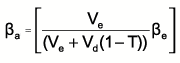
Hence, the asset beta of Moorland will exist a weighted average of these two nugget betas:
ß a (Moorland) = (0.75 × 1.02) + (0.25 × 0.92) = 1.00
Moorland Co disinterestedness beta
So, regearing this asset beta now gives:
1.00 = ßdue east × [l/(50 + l(one-0.xxx))]
So, ße = ane.00/0.59 = 1.69
Moorland Co cost of disinterestedness
Using CAPM:
Kdue east = RF + ß (E(RM) - RF) = 3% + (1.69 × half dozen%) = xiii.ane%
Exam your understanding 2
Using K+K's Suggestion 2 equation, we tin degear the existing thoue and then regear it to the new gearing level:
Degearing:
ke = one thousande i + (1-T)(ke i - kd )(Vd / Ve)
12% = one thousande i+ (1-0.30)(keast i - 4% )(twenty / 80)
Rearranging carefully gives thoudue east i =10.8%
Now regearing:
ke = 10.viii% + (one-0.xxx)(10.8%-4%)(25/75)
ke = 12.four%
Test your understanding 3
From the table the credit spread for an AA rated, 3-yr bond is 30. The spread for a 5-yr bond is 37.
This would advise an adjustment of:
30 + (37 - 30)/ii = 33.five basis points
The yield is therefore establish by calculation 0.335% to the yield on equivalent treasury bonds.
So yield on F’s bonds
2.6% + 0.335% = two.935%
The price of debt = 2.935 × (1 â€" 0.3) = two.05%
Test your understanding 4
The overall cost of debt will exist the weighted boilerplate of the costs ofthe two types of debt (weighted co-ordinate to market values).
ii year bonds
Market value = $30m × 0.90 = $27m
kd = 2.5% + l credit spread (from table) = iii.00%
10 twelvemonth bonds
Market value = $50m × one.08 = $54m
kd = 2.5% + 75 credit spread (from table) = 3.25%
Overall price of debt
Therefore the weighted average price of debt (given that the ratio of market values is 1:2) is
[((1/3) × iii.00%) + ((2/iii) × three.25%)] × (1-0.30) = ii.22%
Test your agreement 5: WACC

Workings:
From CAPM, ke =Rf + ßi (E(Rm) - Rf) = 6% + (1.25 × 8%) = 16%
Ve = $2,500,000 × one.22 / 0.fifty = $6.1m
kd (yield on debt) = risk free rate + credit spread = six% + 65 basis points = 6.65%
Hence, postal service taxation toll of debt = 6.65% (1-0,thirty) = 4.66%
Vd = $ane,000,000 × 110/100 = $1.1m
Therefore, WACC = (6.1 / 7.two) × sixteen% + (ane.1 / 7.2) × 4.66% = 14.three%

| Created at 5/24/2012 3:50 PM by Arrangement Account (GMT) Greenwich Mean Time : Dublin, Edinburgh, Lisbon, London |
Terminal modified at 5/25/2012 12:55 PM by System Account (GMT) Greenwich Mean Fourth dimension : Dublin, Edinburgh, Lisbon, London
| |
| |
| |
Rating : | ") Ratings & Comments (Click the stars to charge per unit the page) Ratings & Comments (Click the stars to charge per unit the page) |
| |
Tags: | |
0 Response to "• What is the best way to minimize the weighted average cost of capital?"
Post a Comment